How to Use Circular References in ExcelCheck, Look For, Enable, or Disable Them
This Excel guide will provide you with the fundamentals of Circular Reference and its importance.
In addition to this, you will as well gain an understanding of how to inspect, locate, and eliminate Excel circular reference (ECR) spreadsheets, along with navigating and enabling circular formulas in circumstances where none of the choices stated above are viable.

Have you arrived at this page because an Excel formula you entered isn’t working as it should? Did you, for example, get an error message pertaining to a circular reference instead of the expected output?
Every day, many users run into similar problems when attempting to make a formula in Excel, and perform its own unique cell computation. This action results in an error message that prompts:
“Careful, we found one or more circular references in your workbook which might cause your formula to calculate incorrectly.”
In simpler terms, Excel is saying, “Hey, I might get stuck in a loop; do you still want this to continue?”
Circular references in Excel are clearly problematic.
Therefore, it’s generally a good idea to stay as far away from them as you can. But in some cases, using an Excel circular reference might be the only practical way to complete the task at hand.
How to Define an Excel Circular Reference
Microsoft has given a clear and concise explanation of what a circular reference is: “If an Excel formula creates a reference to itself or its own cell, whether directly or not, it results in an Excel’s circular reference.”
By way of example, entering the formula =A1 into cell A1 would cause an ECR.
Similarly, inputting any alternative formula and/or calculation that refers to A1, such as =A1*5 or =IF(A1=1, “OK”), would result in the same outcome.
You will see the following alert when you press Enter then the formula will be completed:
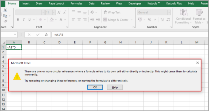
Circular references in Excel have the ability to cycle indefinitely, then create an unending loop that can drastically slow down workbook calculations. Microsoft Excel issues a warning about this.
In some circumstances, a formula that has a circular reference may successfully complete before attempting to calculate its own, resulting in Microsoft Excel returning the same value from the prior successful computation.
After receiving the aforementioned warning, you may click on assistance for more details, or dismiss the dialog box that appears when selecting either the cross button or OK a circular excel reference.
Note: Excel won’t often display the error message repeatedly when you enter multiple formulas with circular excel references.
It is easy to unintentionally construct a circular reference in your Excel sheet, despite the fact that no sensible user would purposefully enter an Excel circular formula the same as the one stated above. As an example, consider the following:
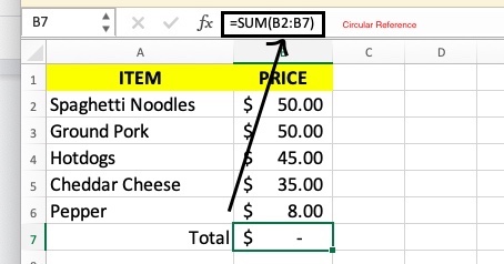
Say you want to use the SUM formula to add the numbers in a column (column A for example), but you unintentionally include the whole cell of its own (B6 in the example).
You will get the error message mentioned earlier in case circular references in Excel are forbidden, which is the default configuration. Your circular formula will yield 0 if iterative or repetitive calculations are enabled, as demonstrated in the accompanying screenshot:
At times, at least one blue arrow may suddenly show in the spreadsheet, making you believe that your Excel program is malfunctioning and may crash.
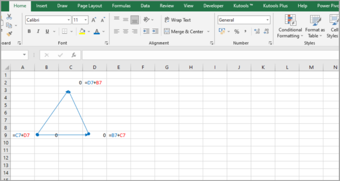
However, these arrows are simply Trace Dependents and/or Trace Precedents, indicating which cells impact or are impacted by an active cell. We will cover how to display and conceal these arrows shortly.
At this point, you may have formed the notion that circular references in Excel are entirely pointless and risky, and may be curious as to why Excel hasn’t prohibited them entirely.
However, as previously stated, there are extremely uncommon scenarios in which the use of circular reference can be valid since it can offer a more concise and sophisticated solution or answer if there’s anything else that will work. The subsequent example serves as a demonstration.
An Example of Using Circular References in Formulas
Here is a typical scenario involving circular references: Consider a scenario in which you have an inventory of objects under column A and the delivery status under column B. You may prefer the timestamp to be inserted automatically as a fixed, unchanging timestamp, the same row under column C when “Yes” is typed in column B.
It is not possible to use a straightforward NOW() formula since this type of Excel function is volatile – meaning that it alters its value whenever the worksheet is reopened or recalculated. One possible solution is to incorporate the nested IF function in the second statement accompanied by a circular reference.
=IF(B2=”yes”, IF(C2=””, NOW(), C2), “”)
B2 in this formula stands for the status of delivery, and C2 on the other hand is the field into which the timestamp should be entered.
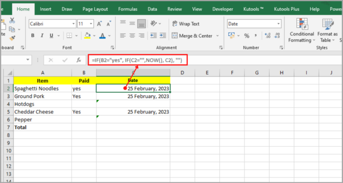
In the formula above, the first function of IF checks to see if cell B2 has the required text, “Yes,” or other text entered in the formula.
The second function of IF is called if the supplied text is present. If not, it returns a blank string.
In order to preserve all prior time stamps, the second function of IF, which is Excel’s circular formula, only retrieves the current date and time if cell C2 is empty.
Note: You must permit iterative calculations in your worksheet for this Excel circular formula to function. This is precisely what we will cover in the section that follows.
How to Turn Excel’s Iterative Calculations On or Off
As mentioned earlier, Excel typically has iterative calculations turned off by default.
To make circular formulas work, you need to allow iterative formulations in your Excel spreadsheet.
To do this, you can use Excel 2010 or the newer versions and follow these steps:
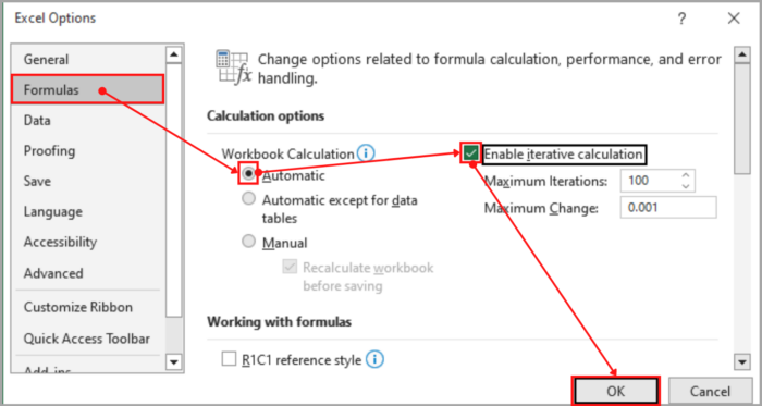
> Click on the File menu and select Options.
> In the left-hand window of the dialog window for Excel Options, choose Formulas.
> In the section of Calculation categories, check the box next to iterative calculation (Enable).
> Optionally, you can adjust the maximum iterations’ number and the amount of change between iterations.
> Click OK to save the changes.
The Reasons for Avoiding Circular References
Using Excel’s circular references is generally discouraged due to performance problems and an error message that appears every time the workbook is opened (only if iterative calculations have been enabled).
Furthermore, circular references may lead to various other problems that may not be immediately evident.
For instance, if you inadvertently switch to “formula editing” by pressing the F2 button or clicking a cell twice with a circular reference, and then selecting Enter without changing the formula, then it will go back to zero.
Therefore, a lot of respected Excel experts recommended avoiding in sheets the use of circular references whenever feasible.
Process for Identifying Excel’s Circular References
To verify if the Excel workbook contains circular references, follow these steps:
On the tab for Formulas, you can click on the arrow right next to Error Checking, then hover over Circular References.
This will display the most recently used circular reference.
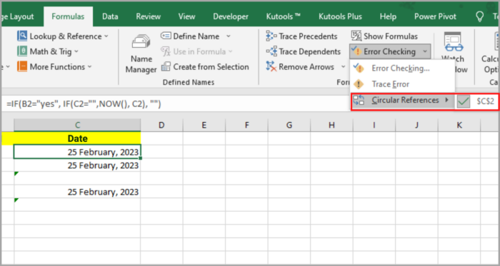
Excel will transport you immediately to the cell that is listed under Circular References when you click on that cell.
The status bar will now alert you that your worksheet has circular references and show the address of one of those cells.
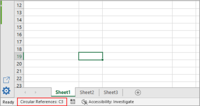
Note: When the Iterative Calculation option is turned on, it is not possible to show the cell that includes a circular excel reference in the status bar. Hence, before attempting to examine the worksheet for circular references, disable it.
Removing Excel’s Circular Reference
Unfortunately, there isn’t an automatic solution to instantly delete all circular formulas from an Excel workbook.
The circular formula must be manually examined by doing the aforementioned processes, and you must then decide whether to completely eliminate the circular formula or replace it with one simpler formula.
Sadly, Excel lacks a function that enables you to instantly delete all circular formulas from a workbook.
The circular formula must be deleted or replaced with one or simpler formulas after carefully inspecting each circular reference using the above-described processes.
How to Identify Connections Between Cells and Formulas
The Trace Precedents and Trace Dependents tools in Excel can shed light on Excel circular references if they are not immediately evident.
These tools use lines to show which cells the selected cell influences or is influenced by.
To show the trace arrows in Excel:
- Navigate to the Formulas tab.
- Then, the Formula Auditing group.
- Lastly, select one of the following options:
- The Trace Precedents feature in Excel traces cells that provide data to a formula and draw lines to indicate which cells affect the selected cell.
- The Trace Dependents feature traces of cells that are dependent on the active cell and show which cells contain formulas that reference the selected cell by drawing lines to indicate which cells are affected by the selected cell.
As an alternative, you can use these shortcuts:
- Trace Precedents: Alt+T U T
- Trace Dependents: Alt+T U D
Click the Remove Arrows button, which is located immediately beneath Trace Dependents, to make the arrows invisible.
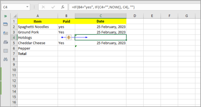
The cells that directly supply data to B6 are shown by the Trace Precedents arrow in the aforementioned example.
As you can see, the calculation returns 0 because cell B6 is also referenced, resulting in a circular excel reference.
Fortunately, changing B6 to B5 in the parameter of the SUM calculation will solve this problem quickly: =SUM(B2:B5).
Some circular references might not be as obvious and can call for more research and calculations.
This is how you handle circular references in Excel.
This quick instruction should have shed some light on this “blind spot,” and you may now do an extra study to find out more.
