Adding Ranks to Pivot Tables in Excel3 Methods with Tutorial with Screenshots
One advantage of pivot tables is the ability to summarize data effectively, making it easier to analyze by categorizing and grouping information such as products, months, etc.
A popular technique for evaluating data is ranking, which enables comparison between categories and products by determining their positions.
With the use of ranking in pivot tables, time and effort can be saved while improving the overall analysis process.
In this post, we will discuss three methods to incorporate a ranking column into pivot tables.
Please note that pivot tables belong to the intermediate category of Excel skills while incorporating ranking within pivot tables is considered to be an advanced proficiency in the use of pivot tables.
Incorporating a Ranking Column in Pivot Tables for Excel 2010 and Later Versions
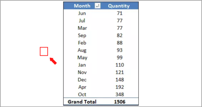
- To calculate ranking in a pivot table, duplicate the value field.

- Right-click on any cell in the second data column.
- Access the “Show Values As” option from the menu. Choose either “Rank Smallest to Largest” or “Rank Largest to Smallest” as desired.

- This will transform the column values into ranks, which can then be sorted for easier analysis of the ranking.

If you are using Excel 2010 or an earlier version, this is the simplest way to incorporate ranking into your pivot table.
It is crucial to note that when filtering the pivot table, the ranks will be altered using this method.
Incorporating a Ranking Column in Pivot Tables for Excel 2007 and Older Versions
- Start by arranging the data in ascending order for which the ranking is to be calculated.

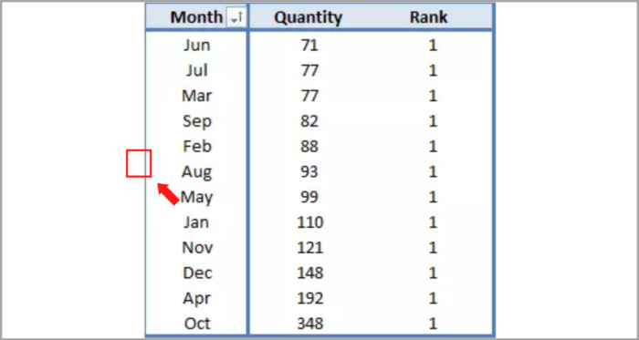
- Open the calculated field dialog box and enter “=1” in the formula input bar.

- This will add a new field to your pivot table with a value of 1 in every cell.

- Right-click on any cell in the newly created field.
- Choose the “Value Field” option and navigate to the “Show Values As” tab in the value field settings dialog box.
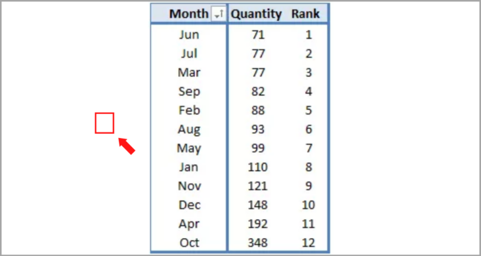
- Select “Running Total In” from the drop-down list and click OK.

- Your pivot table will now display a column with the rankings.

Attention: Ensure that the pivot table has been sorted in ascending or descending order before proceeding.
Employing RANK.EQ and RANK.AVG in the Source Data
While this method may require some effort, it is highly efficient. The benefits of using RANK.EQ and RANK.AVG is that no additions are necessary to the pivot table. Simply follow these easy steps.
Simply follow these steps.
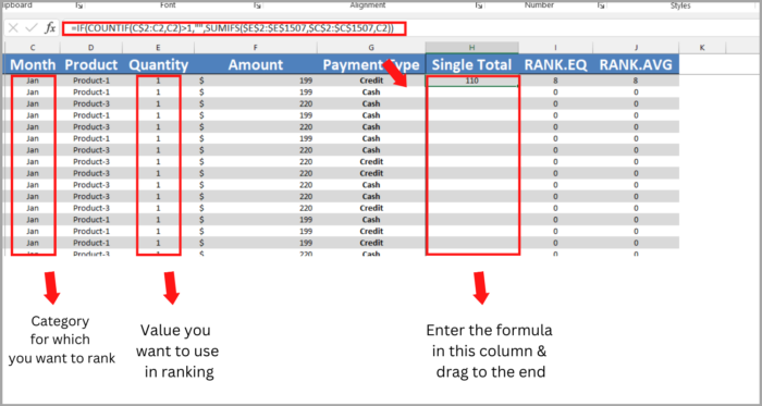
- Begin by inserting a new column in the raw data and entering this formula into the formula bar:
- =IF(COUNTIF(C$2:C2,C2)>1,””,SUMIFS($E$2:$E$1507,$C$2:$C$1507,C2))
- (Here’s how the formula operates: it will generate a single total for each category in the column, which can be used to determine the rank for each category).

- Next, insert two additional columns at the end of the data and apply the following formulas to them.
- =IF(H2=””,0,RANK.EQ(H2,$H$2:$H$1507,1))
- =IF(H=””,0,RANK.AVG(H2,$H$2:$H$1507,1))
- (Here’s how the formula functions: RANK.EQ and RANK.AVG calculates the rank for each category in the data set. Both of these functions are utilized to obtain various ranking types).
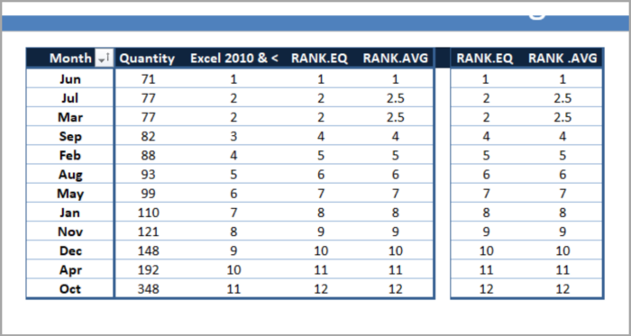
- Afterward, create a pivot table from this data, similar to the following. Either of the two columns can be used to calculate the ranking.

- Note: When utilizing this technique, the ranking will remain unchanged when you filter the items.
Inserting a Separate Ranking Column in a Pivot Table
Alternatively, a manual rank column can be added to a pivot table instead of relying on formulas or other methods.
This approach is useful for instances where a separate ranking is desired. Here are the straightforward steps to follow.
- Create a pivot table and sort the values in either ascending or descending order according to your preference.

- Add the following formulas in two columns that are adjacent to your pivot table.
- Fill the columns with the formulas and the ranking will be displayed in line with your pivot table.

I hope this helps you a lot!


