Easy Steps to Add Total Row in Excel TableStep by Step Instructions with Screenshots
Tables in Excel provide some of the features that you can easily use.
By using an Excel table, organizing and viewing data is done easily in a tabular format.
This will conveniently summarize the data for each column by adding a ‘Total row’ in your table.
In this short tutorial, we will tackle how to convert your given dataset into Excel Table and add a Total Row.
Excel Table
Many users of Excel assume that the data in their spreadsheets are automatically considered as a table since their data is organized into columns and rows.
This is cannot be a ‘Table’ unless you specify it to be one.
An Excel Table is a set of columns and rows that are organized and pre-formatted with features like data styling, aggregation automatic update, and many more.
A Total Row gives you a summary computation of all the data in your column, Total Row is a somewhat form of data aggregation.
Examples of this are average, sum, count, etc.
How to Convert your Dataset into an Excel Table
Your data should be first converted to an Excel Table to view the Total Row.
Consider the given data set in the image below as an example:

Here’s the step-by-step process of how to convert the dataset into an Excel Table:
- First, you need to click any cell in your dataset.
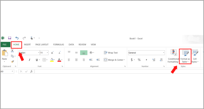
- Go to the Home tab. In your Style group, select ‘Format as Table’.

- A drop-down menu will appear and select what style you want.

- After this, the ‘Format as Table’ dialog box will appear.
- Now, check if your dataset is in the range of the table you want to create is correct. This is under ‘where is the data for your table’.

- You will now see your selected data is wrapped by a green marching ant box. Redo this action if the range is not covering your data.

- Make sure the ‘My table has headers’ box is checked if your data has a header (if not, you are not required to check this).
- Lastly, click the OK button.
Note:
Instead of doing steps 2 and 3, you can use the CTRL+T (keyboard shortcut).
You can now see that your dataset is now converted to an Excel Table.
You can confirm this if your table has small arrows in the top row or header row and the style of the dataset is changed.
How to Add a Total Row to your Excel Table
Since you are done converting your dataset to an Excel Table, Total Row can now be easily added to your Excel Table. You can do this in two easy ways.
Method 1
- First, you need to click on any cell in your dataset.
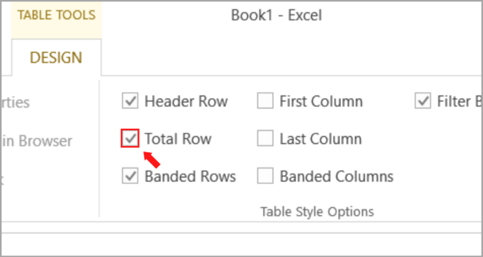
- Go to the Design tab (under Table Tools).

- You will see the Total Row (Under the Table Style Options group).
- Click the box next to the Total Row. This action will display a check inside the box.

Method 2
- In your Excel Table, press right-click anywhere.

- A popup menu will appear, click the Table option.

- From the sub-menu that appears, click the Total Rows.
For either of the two methods you choose, the Total Row will appear at the bottom of your Excel Table (with the total for the last column).

Once you are done adding the Total Row, you may configure it depending on the data that you need. Other than the total, you can choose from the dropdown menu the data you want to show.

How to use other Aggregating Functions in the Total Row
Other aggregating functions can be displayed in the ‘Total Row’ like the max and min, the average, the Standard deviation, and many more.
For example, you need to display the Average Selling Price. Here are the steps on how you can do this:
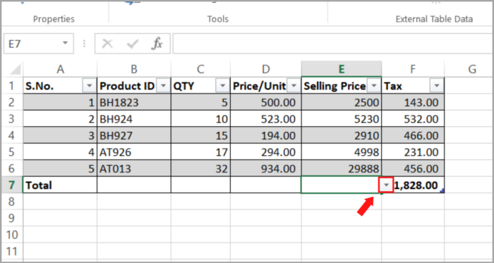
- In the Total Row, select the cell that corresponds to the Selling Price column (cell E7).
- There is an arrow that will appear in the cell that you selected, click that arrow.

- Click the Average option from the drop-down menu that appears.

Now, you can see the Average Selling Price in cell E7.
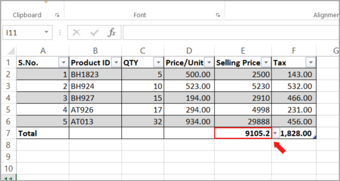
You will see the formula of the average Selling Price in the formula bar of the cell. The Total Row automatically adds the formula.
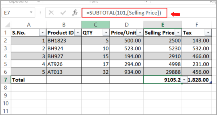
The SUBTOTAL function can ignore even the hidden rows. Even if the table is filtered, the calculated aggregates will be updated correctly.
Remember that the functions are editable, so you can tweak the formula to your liking.
If you want to find the sum of the QTY, you can use the SUMIF function. You can also use other functions in the drop-down menu.
Here is the step-by-step process for finding the conditional sum of QTY:
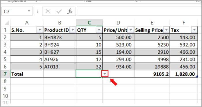
- In the Total Row, select the cell that corresponds to the QTY column (cell C7).
- There is an arrow that will appear in the cell that you selected, click that arrow.

- Click the ‘More Function’ from the drop-down menu that appears.

- The ‘Insert Function’ dialog box will appear, here you can select any available function you want to use.

Conclusion
The Excel Tables help you to make your work easier and quicker to compute your desired result based on your given data.
The Total Rows has many available functions for you to use. There are different aggregating functions you can choose depending on the requirement of your project.
We hope this tutorial has helped you.

