How To Add, Remove, Change, and Print Gridlines in ExcelStep by Step Instructions with Screenshots


In Excel, gridlines are the lines that divide the cells from each other in worksheets.
These lines help users to distinguish between cells, thus making it easier to read the data in the cells.
This might sound like borders, but gridlines are different from borders.
Gridlines can be viewed only on the whole worksheet.
In contrast, you can choose to apply borders to the whole worksheet or just a specific part of a worksheet.
Essential Points
- Gridlines are useful in Excel. They help to define the boundary of a cell, which also can help to keep the data in the cells separate.
- Gridlines are the lines that separate cells and columns on a worksheet. Microsoft Excel and Google both use gridlines.
- In Excel, gridlines are primarily used to separate the data in the cells. These lines make it easy to organize data.
Next, we will explain how to add, remove, change, and print gridlines in Excel.
Adding Gridlines in Excel
It is not difficult to add gridlines in Excel, and here are the steps you need to take to do so.
- Look at the Excel toolbar and find the “View” tab.

- Then, find the “Gridlines” section.

- Once you check the “View” box in the “Gridlines” section, you should be able to see gridlines on your worksheet.
Removing Gridlines in Excel
Gridlines are visible in Excel by default, so if you don’t want them to be visible.
Here is how to remove them from your worksheet.
- Find the tab “Page Layout.”
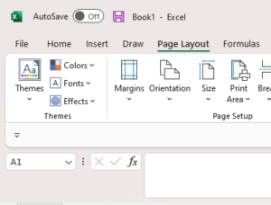
- Next, look for the “Sheet Options Group.”
- Then, find “Gridlines” and remove the check mark from the “View” box.

You should now find that the gridlines are removed from the worksheet.
Using a Gridline Effect in Specific Areas of Your Worksheet
There may be times when you would like to have gridlines in only a particular part of a worksheet.
Unfortunately, in Excel, you either have gridlines in your whole worksheet or none of it. You do not have the option of displaying these lines in only one part of your worksheet.
However, you can use borders that can make it look as if you have gridlines in a particular section of your worksheet.
You have a lot of options when using borders. So, you can choose options that will make the borders look just like gridlines.
Also, you won’t have any problems with printing since these lines are always printed.
Just as you may want to have gridlines in only a particular part of your worksheet, there could be times when you want to hide the gridlines in specific cells. Here is how to do that.
- Select the cells in which you want the gridlines hidden.’
- Now, right-click on the range of cells you just selected and choose “Format Cells” from the menu in the dialog box.

- Then, look for the “Border” tab under “Format cells.”
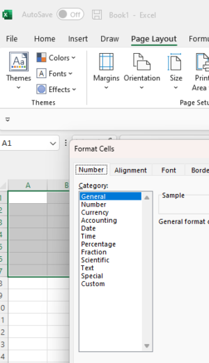
- Next, choose white for the color and then press the buttons “Outline” and “Inside” under the “Presets” option found in the “Border” tab. After this is done, click okay.

After you complete these steps, you should find that the gridlines are hidden for the range of cells you selected.
Choosing Different Colors for Your Gridlines
You do have the option of choosing different colors for your gridlines in your worksheets. Here is how to set the default color for your gridlines.
- Go to “Options” under “File.”
- Now, in the dialog box, choose the “Advanced Option. Choose “Display Options For This Worksheet.”

- Next, Select the color you want for your gridlines from the Gridline Color dropdown.

- Then, choose okay.
This will change the color of your active worksheet.
However, you can change the color of the gridlines for all of your worksheets.
Just press down the Control Key and hold it. Then, select the tabs you want.
The worksheet should now be in Group Mode. So, you can now change the color of the gridlines, and it should be applied to all of your worksheets.
Be sure to ungroup your worksheets now by right-clicking on the tab and choosing ungroup.
This will ensure that other changes you make in your current worksheet won’t be applied to all of your worksheets.
Just remember this does not change the default color of gridlines. The next time you open a workbook or insert a new worksheet, the color of the gridlines will be light gray.
Printing the Gridlines in Your Excel Worksheets
Gridlines in Excel are not automatically printed. This is by default.
But, by following these steps, you can print your worksheet with gridlines.
- Find the “Page Layout” tab in the toolbar and look for the “Gridlines” option.
- Now, in “Sheet Options,” in the “Gridlines” options, place a checkmark in the box for “Print.”
- After print is enabled, you will see the gridlines when you print.
Advantages of Gridlines
- Gridlines are displayed by default, so you don’t have to change any settings for them to appear on your worksheet as you work.
- Gridlines are customizable, including their pattern and color, as well as their thickness.
- You can use the options on your toolbar to hide gridlines.
- Gridlines are useful for keeping your data organized.
Disadvantages of Gridlines
- Gridlines can be difficult for some users to see because of their light color.
- Gridlines are not printed by default in Excel worksheets.
- Gridlines must be displayed in the whole worksheet or not at all, which can be inconvenient if you would like them displayed in only part of a worksheet.
Important Items To Keep in Mind
- When you would like to display or hide gridlines on your worksheet, you can check or uncheck the “Gridlines” option under the “View” tab on the Excel toolbar.
- Another option for displaying or hiding gridlines is to use a keyboard shortcut. Just press “ALT+W+VG” in order to display or hide gridlines on your worksheet.
- You can also hide gridlines by applying a background color to the range of cells where you want to hide the gridlines. Make sure to use the option “No Fill” to your selected cells when applying the background color.
- If you want to display or hide gridlines in more than one worksheet, you can press down the Control key and hold it, then click on the “Sheet” tab. This will allow you to apply the changes you want to your selected spreadsheets.
Final Thoughts
Gridlines are convenient for organizing your data.
But, in some cases, you may want to hide the gridlines or customize them.
So, in this article, we have shown you several options for showing and hiding gridlines, as well as how to customize them.