3 Easy Ways to Convert a Date to Day of the WeekStep by Step Instructions with Screenshots


Having a lot of information in Excel can be overwhelming especially if you do not know how to simplify the data and get only what you need.
This is especially true for data with specific date information; you need to convert the date to determine the day of the week.
Instead of seeing the date, you would want to see a specific day of the week – be it a Monday, Friday, or Saturday.
When dealing with your to-do lists or reports (daily, weekly, or monthly), knowing how to convert a date to a day is helpful.
We will explore the three different ways of converting dates to days of the week in this article.
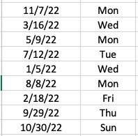
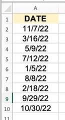
As an example, the below data will be used all throughout the illustrations and converted into days of the week:
The three methods we will use to convert them are the following:
Method 1: Text Function
Method 2: Format Cells Feature
Method 3: Mix of Formulas
Method 1: Text Function
Using this, you will be able to get text formats from the converted dates.
Parts of the date are extracted from the date or date serial number to meet your requirement.
The syntax of the text function is shown as follows:
=TEXT(date,date_format_code)
With the above function, the date refers to the date serial number or the date that needs to be converted, while the date_format_code refers to the format that you wish the date to be.
Using the text function, the date_formate_code will convert the date to the format that you like.
For example, the data in A2 is “11/7/22”. Using the function =TEXT(date,date_format_code), it will then be =TEXT(11/7/22,”dddd”) and will return Monday.
Below are the format codes for the different days or months:
- d – represents one or two digits of the day (1 or 10)
- dd – represents two digits of the day (01 or 10)
- ddd – represents the abbreviated form of the day of the week (Mon, Wed)
- dddd – represents the full name of the day of the week (Monday, Wednesday)
This means then that:
- When =TEXT(11/7/22,”d”) is applied, you will get 7
- When =TEXT(11/7/22,”dd”) is applied, you will get 07
- When =TEXT(11/7/22,”ddd”) is applied, you will get Mon
- When =TEXT(11/7/22,”dddd”) is applied, you will get Monday
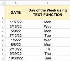
Using the text function and applying this to the sample table we have above, the result will be:
Steps to Convert to Day of the Week Using Text Function
- Click on the cell that you want to convert.
- In the formula bar, enter the formula needed to convert the date to your desired format. For example, =TEXT(A2,”dd”) or =TEXT(A2,”dddd”) and press enter.
- To copy the format to the rest of the cells, simply double-click on the fill handle or drag it down.
- To store the results of the formula sa permanent values, follow these:
- Highlight the cells you wish to copy the formula results. Press CTRL+C OR CMD+C.
- Right-click and from the options that pop up, click on Paste Options and then Paste Values.
- You can delete Column A without the formula results changing.
Using the above steps, you will see the column with the converted values as shown below:
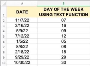
It must be noted that the results in Column B will differ depending on the format code used.
Method 2: Format Cells Feature
This feature is a more straightforward way of converting the dates to your preferred days of the week without the need for a new column to type the formula.
You can go ahead and replace the data from the same column.
Steps:
- Select the cells you wish to convert.
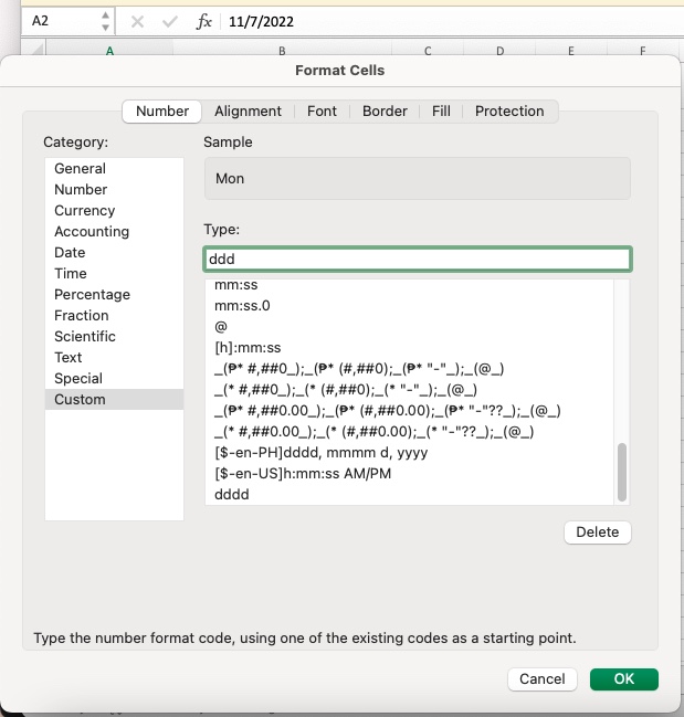
- Right-click and from the pop-up menu, click on Format Cells.
- You can also select the Custom option in the Format Cells dialog box when selecting the dialog box launcher in the Home Tab > Number group.
- Under Category, click on Custom.
- Under type, select the formatting type you wish to convert your date into. Click OK to close the dialog box.
Method 3: Mix of Formulas
When you are more comfortable writing your own formula, that can also be possible to convert the dates to days.
There are two functions that are to be used: the Weekday Function and the Choose Function.
Weekday Function
Using this function, the dates can be converted to days that start from 1 to 7, depending on the beginning day of the week.
This is especially helpful when it comes to some countries that start their day on Sunday or Saturday in the case of countries in the Middle East.
The Weekday Function’s syntax is shown as:
WEEKDAY(date, [type])
Where:
- Date = a date or a date serial number, or a cell reference that stores the date value.
- Type = this parameter is actually optional and determines what day of the week to start from. For example, if the input data is 1, it means the week starts on a Sunday and will end on Saturday. If it is 2, it starts on a Monday, and 3 starts on a Tuesday, and so on. The default value of this parameter is 1.
Using the example above, WEEKDAY (A3, 1) will return the value 4 which corresponds to a Wednesday.
Choose Function
As opposed to the Weekday Function, the Choose Function gives you an alternative to getting the outcome that you want, depending on a value.
For example, you want to show “orange” when the value is 1, or “purple” if the value is 2.
This shows an excellent way of choosing other outputs instead of just the nested IF functions.
The syntax to be used is:
=CHOOSE(index, value1, , …) is an Excel function that returns a value from a list based on the position you specify as the index.
Where:
- Index = a number anywhere between the value of 1 – 254
- Value1 = first value of the possible outputs based on the list
- Value2 = first value of the possible outputs based on the list
Using the syntax above and the example given, =CHOOSE (2, “sun”, “mon”, “tue”, “wed”, “thu”, “fri”, “sat”) will give an output of Monday because it is the second value based on the list provided.
Putting the Formula Together
When we put the Weekday and Choose Function together, we can follow the following steps:
- Select the cell that you wish to see the output of the formula.
- Type in the formula: =CHOOSE(WEEKDAY(A2), “Sun”, “Mon”, “Tue”, “Wed”, “Thu”, “Fri”, “Sat”)
- Click enter.
- You will be able to see the day of the week in your chosen cell. To copy the formula to the rest of the cells below it, simply click on the cell, and copy and paste. Or you can also drag it down.
- To store the formula, right-click on the cell and click > Paste Options > Paste Values.
- You can delete the data in Column A and keep the values in column B.
Below will be the result from the steps above: